MIT6.006 NOTES

Lecture 01 (Algorithms and Computation)

• Algorithm: Procedure mapping each input to a single output (deterministic)
• Correctness:

  • For small inputs, can use case analysis
  • For arbitrarily large inputs, algorithm must be recursive or loop in some way
  • Must use induction (why recursion is such a key concept in computer science)

• Efficiency: Count number of fixed-time operations algorithm takes to return

  Asymptotic Notation: ignore constant factors and low order terms
  

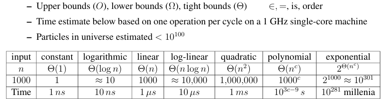
• Model of Computation

  • Specification for what operations on the machine can be performed in O(1) time
  • Model in this class is called the Word-RAM

• Data Structure:

  • A data structure is a way to store non-constant data, that supports a set of operations
  • A collection of operations is called an interface

Lecture 02 (Data Structures and Dynamic Arrays)

• Interface(what you want to do) vs Data Structure(how you do it)

• Interface:

  • specify what data you can store
  • A set of operations that can be performed on a data structure
  • problem

• Data Structure:

  • actual representation of the data
  • tells how to store the data
  • gives algorithm for each operation in the interface
  • solution

2 main Interfaces

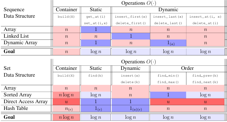
Sequence

Static sequence interface: fixed size, can only access elements by index

• build(n): create a sequence of size n
• len(): return length of sequence
• iter_seq(): iterate through sequence
• get_at(i): return element at index i
• set_at(i, x): set element at index i to x
• get_first/last(): return first/last element
• set_first/last(x): set first/last element to x

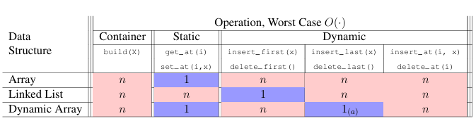
• Static array: fixed size, contiguous block of memory

  • array[i] = memory[address(array) + i * size_of_element]
  • O(1) per get_at(i)/set_at(i, x)/len() (assume w $\ge \lg(n)$ ， 机器字可以容纳所有可能的下标值 i，CPU 能在一步内完成寻址和访问，保证操作是 O(1))
  • O(n) per build(n)/iter_seq()
  • insert of array is O(n) (need to shift elements), not allowed to be bigger, so need to allocate a new array and copy

Dynamic sequence interface: variable size, can only access elements by index

• insert_at(i, x): insert x at index i
• delete_at(i): delete element at index i
• insert/delete_first/last(x): insert/delete at beginning/end of sequence

• Linked lists: each element points to the next element in the list

  • get/set_at(i) need O(i) time
  • data structure augmentation: store the address of tail

• Dynamic Arrays(lists in Python):

  • relax constant size(array) = n
  • enforce the size of array = $\Theta(n)$ & $\ge n$
  • maintain A[i] = $x_i$
  • insert_last(x): set A[len] = x; len += 1 (iff len < size(A))
  • when len = size(A), double the size of A, copy elements to new array, the resize and copy costs is linear each time, in total $\Theta(n)$ (Amortization: average cost per operation over a sequence of operations)

Lecture 03 (Sets and Sorting)

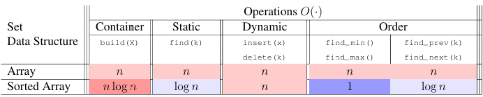
Set Interface

• Container:

  • build(A): given an iterable X, build set from items in X
  • len(): return the number of stored items

• Static Set:

  • find(k): return the stored item with key k

• Dynamic:

  • insert(x): add x to set (replace item with key x.key if one already exists)
  • delete(k): remove and return the stored item with key k

• Order:

  • iter_ord(): return the stored items one-by-one in key order
  • find_min(): return the stored item with smallest key
  • find_max(): return the stored item with largest key
  • find_next(k): return the stored item with smallest key larger than k
  • find_prev(k): return the stored item with largest key smaller than k

Sorting

• Vocabulary:

  • Destructive: sorts in place, modifies the input sequence
  • In place: uses O(1) additional space, only uses a constant amount of extra memory

Permutation Sort

def permutation_sort(A):         
    for B in permutations(A):    # O(n!)
        if is_sorted(B):         # O(n)
            return B             # O(1)

$\Omega(n! * n)$

Selection Sort

def selection_sort(A, i = None):       # T(i)
  '''Sort A[:i + 1]'''
  if i is None: i = len(A) - 1         # O(1)
  if i > 0:                            # O(1)
    j = prefix_max(A, i)               # S(i)
    A[i], A[j] = A[j], A[i]            # O(1)
    selection_sort(A, i - 1)           # T(i-1)

def prefix_max(A, i):                  # S(i)
  '''Return index of max in A[:i + 1]'''
  if i > 0:                            # O(1)
    j = prefix_max(A, i - 1)           # S(i-1)
    if A[j] >= A[i]:                   # O(1)
      return j                         # O(1)
  return i                             # O(1)

$\Theta(n^2)$

Insertion Sort

def insertion_sort(A, i = None):      # T(i)
  '''Sort A[:i + 1]'''
  if i is None: i = len(A) - 1        # O(1)
  if i > 0:                           # O(1)
    insertion_sort(A, i - 1)          # T(i-1)
    insert_last(A, i)                 # S(i)
    
def insert_last(A, i):                # S(i)
  '''Sort A[:i + 1] assuming sorted A[:i]'''
  if i > 0 and A[i] < A[i - 1]:       # O(1)
    A[i], A[i - 1] = A[i - 1], A[i]   # O(1)
    insert_last(A, i - 1)             # S(i-1)

$\Theta(n^2)$

Merge Sort

def merge_sort(A, a = 0, b = None):       # T(b - a = n)
  '''Sort A[a:b]'''
  if b is None: b = len(A)                # O(1)
  if b - a > 1:                           # O(1)
    c = (a + b + 1) // 2                  # O(1)
    merge_sort(A, a, c)                   # T(n / 2)
    merge_sort(A, c, b)                   # T(n / 2)
    L, R = A[a:c], A[c:b]                 # O(n) 
    merge(L, R, A, len(L), len(R), a, b)  # S(n)

def merge(L, R, A, i, j, a, b):           # S(b - a = n)
  '''merge sorted L[:i] and R[:j] into A[a:b]'''
  if a < b:                               # O(1)
    if (j <= 0) or (i > 0 and L[i - 1] >= R[j - 1]):  # O(1)
      A[b - 1] = L[i - 1]                 # O(1)
      i = i - 1                           # O(1)
    else:
      A[b - 1] = R[j - 1]                 # O(1)
      j = j - 1                           # O(1)
    merge(L, R, A, i, j, a, b - 1)        # S(n - 1)

$\Theta(n \log n)$

T(n) = 2T(n/2) + O(n)

Lecture 04 (Hashing)

• Can find(k) be faster than O( $\log n$ )?

  NO!

Comparison Model

• Comparison is the only way to distinguish between elements (=, <, >, ≤, ≥, ≠)
• Any searching decision tree has at least (n+1) leaves, so it has at least $\log_2(n+1)$ height, so running time of any comparison-based algorithm is at least $\Omega(\log n)$
• More generally, height of tree with $\Theta (n)$ leaves and max branching factor b is $\Omega(\log_b n)$
• To get faster, need an operation that allows super-constant $\omega (1)$ branching factor. How?

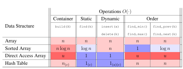
Direct Address Array

• Exploit Word-RAM O(1) time random access indexing, linear branching factor
• Space complexity is O(u) for the biggest key u
• If keys fit in a machine word, i.e. $u \le 2^w$ , then we can use a direct address array

Hashing

• Idea: If $n \le u$ , map keys to a smaller range $m = \Theta (n)$ and use smaller direct access array
• hashing function: $h(k): \{0, ..., u - 1\} \to \{0, ..., m - 1\}$ to map keys to indices
• Direct access array called hash table, h(k) called the hash of k
• If $m \ll u$ , no hash function is injective by pigeonhole principle, so collisions are inevitable (always exists keys h(a) = h(b) for a ≠ b)

  Deal with collisions:

  • Chaining: Store a linked list of keys at each index of the hash table

  vector<pair<int,int>> table[m]; // 每个槽位是一个 vector

  • Open addressing: Store keys directly in the hash table, find next available slot for a key that collides with an existing key
    • complicated analysis, but common and practical

  struct Entry {
      int key;
      int value;
      bool occupied;
  };
  
  Entry table[m]; // m 大小的数组

Chaining

• Store collisions in another data structure (a chain)
• If keys roughly evenly distributed over indices, chain size is n/m = n/ $\Omega (n)$ = O(1), and find(k) is O(1) on average
• If not evenly distributed, chain size can be O(n), and find(k) is O(n) in the worst case

Hashing Function

Devision (bad): h(k) = k mod m

• Heuristic, good when keys are uniformly distributed
• m should avoid symmetries of the stored keys
• Large primes far from powers of 2 and 10 can be reasonable
• (Python uses a version of this with some additional mixing )
• If $u \gg n$ , every hash function will have some input set that will a create O(n) size chain
  • Don’t use a fixed hash function! Choose one randomly (but carefully)!

Universal (good, theoretically): $h_{ab} (k) = (((ak + b) \mod p) \mod m)$

• Hash Family: $\mathcal{H} (p, m) = \{ h_{ab} | a, b \in \{ 0, ..., p - 1 \} \text{ and } a \neq 0 \}$
• Parameterized by a fixed prime p > u, with a and b chosen from range {0,...,p − 1}
• $\mathcal{H}$ is a Universal family: ${Pr}_{h \in \mathcal{H} } \{ h(k_i) = h(k_j) \} \le 1/m$ $\forall k_i \neq k_j \in \{ 0, ..., u - 1 \}$ (两个不同的 key 发生冲突的概率 ≤ 1/m)
• $X_{ij}$ indicator random variable over $h \in \mathcal{H}$ : $X_{ij} = 1$ if $h(k_i) = h(k_j)$, else $X_{ij} = 0$
• Size of chain at index $h(k_i)$ is $X_i = \sum_{j} X_{ij}$, so $E[X_i] = \sum_{j} E[X_{ij}] = 1 + \sum_{j \neq i} E[X_{ij}] \le 1 + (n - 1) / m$
• Since $m = \Omega(n)$ , load factor $\alpha = n/m = O(1)$, so $E[X_i] = O(1)$

Dynamic Hashing (m is not fixed)

• 当 负载因子 n/m (0.5 ~ 0.75 is ideal) 偏离 1 太多时（过大或过小），需要：

  • 重新选择一个随机哈希函数
  • 调整表的大小 m，并重建哈希表

• 这种重建操作类似于 动态数组的扩容/缩容：

  • 单次重建开销较大
  • 但其代价可以分摊（amortized）到多次插入/删除操作上

• 因此：

  • 哈希表支持的动态集合操作（如 insert、delete、search）
  • 在 期望的摊还复杂度 下，依然保持 O(1) 时间

Problem Session 2

Recursion Tree

• Recursion tree is a tree representation of the recursive calls made by an algorithm
• Each node represents a recursive call, and the edges represent the recursive calls made by that call
• By summing the work done at each level of the tree, we can estimate the total running time of the algorithm
• The recursion stops at the leaves, when the subproblem size becomes constant
• 系数是叶子数，括号内的是每个叶子的工作量

Example 1:

$T(n) = 2T(n/2) + n$

• Level 0 (root): cost = $n$
• Level 1: 2 subproblems of size $n/2$, cost = $2 \cdot (n/2) = n$
• Level 2: 4 subproblems of size $n/4$, cost = $4 \cdot (n/4) = n$
• ...
• Level $\log_2 n$: cost = $n$
• Total cost: $n + n + n + \dots + n = n \log n$

$T(n) = \Theta(n \log n)$

---

Example 2:

$T(n) = 3T(n/2) + n^2$

• Level 0 (root): cost = $n^2$
• Level 1: 3 subproblems of size $n/2$, cost = $3 \cdot (n/2)^2 = 3n^2/4$
• Level 2: 9 subproblems of size $n/4$, cost = $9 \cdot (n/4)^2 = 9n^2/16$
• ...
• The work per level decreases geometrically.
• The root cost $n^2$ dominates the total.

$T(n) = \Theta(n^2)$

---

Master Theorem

The Master Theorem provides a direct way to analyze recurrences of the form:

$T(n) = a \, T(n/b) + f(n)$

where

• $a \geq 1$: number of subproblems
• $b > 1$: factor by which subproblem size decreases
• $f(n)$: cost of work done outside the recursive calls

Cases of the Master Theorem:

1. Case 1: If $f(n) = O(n^{\log_b a - \epsilon})$ for some $\epsilon > 0$,
   then $T(n) = \Theta(n^{\log_b a})$.

2. Case 2: If $f(n) = \Theta(n^{\log_b a})$,
   then $T(n) = \Theta(n^{\log_b a} \log n)$.

3. Case 3: If $f(n) = \Omega(n^{\log_b a + \epsilon})$ for some $\epsilon > 0$,
   and the regularity condition holds ($a f(n/b) \leq c f(n)$ for some constant $c < 1$),
   then $T(n) = \Theta(f(n))$.

---

Example 1 (same as recursion tree):

$T(n) = 2T(n/2) + n$

• Here, $a = 2, b = 2$. So $\log_b a = \log_2 2 = 1$.
• $f(n) = n = \Theta(n^1)$.
• Case 2 applies.

$T(n) = \Theta(n \log n)$

---

Example 2:

$T(n) = 3T(n/2) + n^2$

• $a = 3, b = 2$. So $\log_b a = \log_2 3 \approx 1.585$.
• $f(n) = n^2 = \Omega(n^{1.585 + \epsilon})$ with $\epsilon \approx 0.415$.
• Case 3 applies.

$T(n) = \Theta(n^2)$

---

✅ 总结：

• Recursion Tree 可以直观理解每一层的工作量。
• Master Theorem 可以快速判定递推的复杂度。
• 两种方法结合使用，既有直观理解，也有快速计算。

Problem 2-4 (merge sort, O( $n \log n$ ))

def get_damages(H): 
  D = [1 for _ in H] 
  H2 = [(H[i], i) for i in range(len(H))] 
  def merge_sort(A, a = 0, b = None): 
    if b is None: b = len(A) 
    if 1 < b - a: 
      c = (a + b + 1) // 2 
      merge_sort(A, a, c) 
      merge_sort(A, c, b) 
      i, j, L, R = 0, 0, A[a:c], A[c:b] 
      while a < b: 
        if (j >= len(R)) or (i < len(L) and L[i][0] <= R[j][0]): 
          D[L[i][1]] += j 
          A[a] = L[i] 
          i += 1 
        else: 
          A[a] = R[j] 
          j += 1 
        a += 1 
  merge_sort(H2)  
  return D 

Lecture 05 (Linear Sorting)

Comparison Sort Lower Bound

Comparison Model

• Comparison model implies that algorithm decision tree is binary (constant branching factor)
• Tree height lower bounded by $\Omega ( \log L)$ , so worst-case time is $\Omega ( \log L)$
• To sort n items, need at least n! leaves (one for each permutation)
• Thus, worst-case time is $\Omega ( \log n!) \ge \log ((n / 2)^{n / 2}) = \Omega (n \log n)$
• So merge sort is optimal in comparison model
• Can we exploit a direct access array to sort faster?

Direct Access Array Sort

• Suppose all keys are unique non-negative integers in range {0, . . . , u − 1}, so n ≤ u
• Insert each item into a direct access array with size u in $\Theta (n)$
• walk down DAA and return items seen in order in $\Theta (u)$

def direct_access_sort(A):
  "Sort A assuming items have distinct non-negative keys" 
  u = 1 + max([x.key for x in A]) # O(n) find maximum key
  D = [None] * u  # O(u) direct access array
  for x in A:     # O(n) insert items 
    D[x.key] = x
  i = 0
  for key in range(u):  # O(u) read out items in order 
    if D[key] is not None:
      A[i] = D[key]
      i += 1

• What if keys are in larger range, like $u = \Omega (n^2) < n_2$
• Idea! Represent each key k by tuple (a, b) where k = an + b and 0 ≤ b < n
• Specifically $a = k // n$ and $b = k \mod n$
• This is a built-in Python operation (a, b) = divmod(k, n)

Tuple Sort

• Item keys are tuples of equal length, i.e. item x.key = (x.k1, x.k2, x.k3, ...).
• Want to sort on all entries lexicographically, so first key k1 is most significant
• How to sort? Idea: Use other auxiliary sorting algorithms to separately sort each key (Like sorting rows in a spreadsheet by multiple columns)
• What order to sort them in? Least significant to most significant! (to preserve order of more significant keys)
• Idea: Use tuple sort with auxiliary direct access array sort to sort tuples (a, b).
• Problem: Many integers could have the same a or b value, even if input keys distinct
• Need sort allowing repeated keys which preserves input order
• Want sort to be stable: repeated keys appear in output in same order as input
• modify direct access array sort to admit multiple keys in a way that is stable

Counting Sort

• Instead of storing a single item at each array index, store a chain, just like hashing
• For stability, chain data structure should remember the order in which items were added
• Use a sequence data structure which maintains insertion order
• To insert item x, insert_last to end of the chain at index x.key
• Then to sort, read through all chains in sequence order, returning items one by one

def counting_sort(A):
  "Sort A assuming items have non-negative keys" 
  u = 1 + max([x.key for x in A]) # O(n) find maximum key 
  D = [[] for i in range(u)]      # O(u) direct access array of chains
  for x in A:                     # O(n) insert into chain at x.key 
    D[x.key].append(x)
  i = 0 
  for chain in D:                 # O(u) read out items in order 
    for x in chain:
      A[i] = x 
      i += 1 

Radix Sort

• Idea: If $u < n^2$ , use tuple sort with auxiliary counting sort to sort tuples (a, b)
• Sort least significant key b, then most significant key a
• Running time for this algorithm is O(2n) = O(n) since $u < n^2$
• If every key < $n^c$ for some positive $c = \log _n (u)$ , every key has at most $c$ digits in base n
• A c-digit number can be written as a c-element tuple in O(c) time
• We sort each of the c base-n digits in O(n) time
• So tuple sort with auxiliary counting sort runs in O(cn) time in total
• If c is constant, this sort is linear O(n)

def radix_sort(A): 
  "Sort A assuming items have non-negative keys"
  n = len(A) 
  u = 1 + max([x.key for x in A])     # O(n) find maximum key
  c = 1 + (u.bit_length() // n.bit_length()) 
  class Obj: pass
  D = [Obj() for a in A] 
  for i in range(n):                  # O(nc) make digit tuples
    D[i].digits = [] 
    D[i].item = A[i]
    high = A[i].key 
    for j in range(c):                # O(c) make digit tuple 
      high, low = divmod(high, n)
      D[i].digits.append(low)
  for i in range(c):                  # O(nc) sort each digit
    for j in range(n):                # O(n) assign key i to tuples 
      D[j].key = D[j].digits[i]
    counting_sort(D)                  # O(n) sort on digit i 
  for i in range(n):                  # O(n) output to A
    A[i] = D[i].item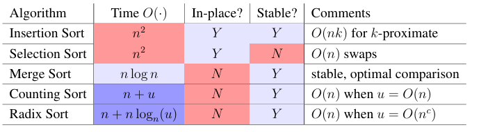

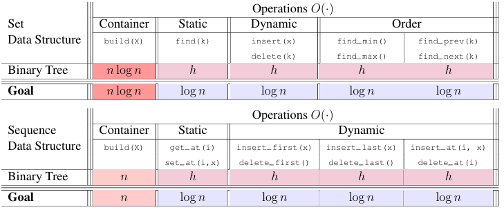
Lecture 06 (Binary Trees I)

Binary Tree

• pointer-based data structure, each node has a parent pointer and two child pointers (left and right) node.{item, parent, left, right}

Terminology

• The root of a tree has no parent (Ex: <A>)
• A leaf of a tree has no children (Ex: <C>, <E>, and <F>)
• Define depth(<X>) of node <X> in a tree rooted at <R> to be length of path from <X> to <R>
• Define height(<X>) of node <X> to be max depth of any node in the subtree rooted at <X> (height of a leaf is 0)
• A binary tree has an inherent order: its traversal order

  • every node in node <X>’s left subtree is before <X>
  • every node in node <X>’s right subtree is after <X>

• List nodes in traversal order (mostly refers to in-order) via a recursive algorithm starting at root:

  • pre-order: visit node, then left subtree, then right subtree
  • in-order: visit left subtree, then node, then right subtree (also called symmetric order)
  • post-order: visit left subtree, then right subtree, then node

Tree Navigation (O(h) time)

• subtree_first(node): return first node in subtree rooted at node (leftmost leaf)

  • if node has no left child, return node
  • else, return subtree_first(node.left)

• successor(node): return next node in traversal order after node

  • if node has right child, successor is subtree_first(node.right)
  • else, go up until we find a node that is a left child of its parent, then return that parent

Dynamic operations

• subtree_insert_after(node, new):

  • if node has no right child, set node.right = new and new.parent = node
  • else, find successor(node) and insert new as left child of that node

• subtree_delete(node):

  • if node has no children, set node.parent.left/right = None
  • if node has one child, splice out node by setting node.parent.left/right = node.left/right and node.left/right.parent = node.parent
  • if node has two children, find successor(node), copy its item to node, and then delete successor(node) (which has at most one child)

  ---

  • if node has no children, set node.parent.left/right = None
  • if node.left: swap node and predecessor(node), then do subtree_delete(predecessor) (recursively)
  • else if node.right: swap node and successor(node), then do subtree_delete(successor) (recursively)

Applications of binary trees:

sequence

• traversal order is the sequence order
• find(i) Could just iterate through entire traversal order, but that’s bad, O(n)
• size(node): returns node.size, the number of node in subtree(node), including node itself, O(1)

  • (Maintain the size of each node’s subtree at the node via augmentation, update sizes on insertions and deletions)

• However, if we could compute a subtree’s size in O(1), we can do better:

  • if i = size(node.left), return node
  • if i < size(node.left), return find(i) in node.left
  • else, return find(i - size(node.left) - 1) in node.right

set

• traversal order is the increasing key order
• subtree_find(node = root, k): start at root, and do binary search, O(h)

  • if node is None, return None
  • if k = node.key, return node
  • if k < node.key, return subtree_find(node.left, k)
  • else, return subtree_find(node.right, k)

Lecture 07 (Binary Trees Ⅱ, AVL)

subtree properties

• sum, product, min, max, gcd, lcm, height, etc. of some feature of all nodes in subtree
• not node's index(which is changing), depth(annoying to maintain)
• local vs global

  • local: can be computed from node and its children (e.g. size, sum, max, min)
  • global: need info outside subtree (e.g. depth)

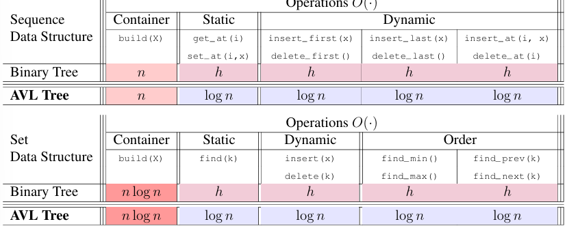
• GOAL: bound h by log(n), maintain a binary tree with height O(log n) to ensure O(log n) time for dynamic operations
• Idea: Use tree rotations to maintain balance
• balanced tree: h = log(n)

AVL Tree

• height-balanced binary search tree
• height balanced:

  • skew(node) = height(node.right) - height(node.left) $\in$ {-1, 0, 1} for all nodes
  • height balanced $\implies$ balanced? why?
    • consider the least balanced tree
    • skew(root) = 1, root: $N_h$, root.left: $N_{h-2}$, root.right: $N_{h-1}$
    • $N_h = 1 + N_{h-1} + N_{h-2} > 2 * N_{h-2} = 2^{\lfloor h / 2 \rfloor} \implies h \le 2 \lg n$

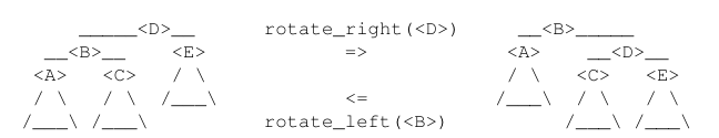
Rotation

• operation to rebalance a binary tree, and preverse the data that's represented by the tree

• accomplished by changing a constant number of pointers:

  • node.parent.left/right = node.right/left
  • node.right/left.parent = node.parent
  • node.parent = node.right/left
  • node.right/left = node.right/left.left/right
  • node.right/left.left/right.parent = node.right/left
  • update heights of affected nodes

• implementation:

  • node.height = 1 + max(height(node.left), height(node.right))
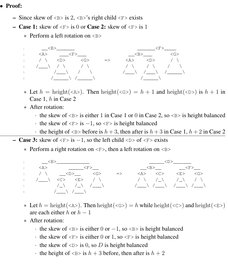
  • whenever insert a new node(only it's ancestor would be effected), consider the lowest out of balance node X, its skew would be 2 or -2
  • if skew(X) = 2, then skew(X.right) = 1 or 0, do left rotation on X
  • if skew(X) = 2, then skew(X.right) = -1, do right rotation on X.right, then left rotation on X
  • verse for skew(X) = -2

  

  Problem Session 4

  4-5

  from Set_AVL_Tree import BST_Node, Set_AVL_Tree
  
  class Measurement:
    def __init__(self, temp, date): 
      self.key = date
      self.temp = temp
    
    def __str__(self): return "%s,%s" % (self.key, self.temp)
  
  class Temperature_DB_Node(BST_Node): 
    def subtree_update(A): 
      super().subtree_update()
      A.max_temp = A.item.temp
      A.min_date = A.max_date = A.item.key 
      if A.left: 
        A.max_temp = max(A.max_temp, A.left.max_temp) 
        A.min_date = min(A.min_date, A.left.min_date) 
      if A.right:
        A.max_temp = max(A.max_temp, A.right.max_temp) 
        A.max_date = max(A.max_date, A.right.max_date)
  
    def subtree_max_in_range(A, d1, d2):
      if (A.max_date < d1) or (d2 < A.min_date): return None
      if (d1 <= A.min_date) and (A.max_date <= d2): return A.max_temp 
      t = None
      if d1 <= A.item.key <= d2: 
        t = A.item.temp
      if A.left: 
        t_left = A.left.subtree_max_in_range(d1, d2) 
        if t_left: 
          t = t_left if t else max(t, t_left)
      if A.right:
        t_right = A.right.subtree_max_in_range(d1, d2) 
        if t_right: 
          t = t_right if t else max(t, t_right)
      return t
  
  class Temperature_DB(Set_AVL_Tree):
    def __init__(self): 
      super().__init__(Temperature_DB_Node)
  
    def record_temp(self, t, d): 
      try:
        m = self.delete(d)
        t = max(t, m.temp)
      except: pass
      self.insert(Measurement(t, d))
  
    def max_in_range(self, d1, d2): 
      return self.root.subtree_max_in_range(d1, d2) 

Lecture 08 (Binary Heaps)

Priority Queue Interface (subset of set)

• build(x): given an iterable X, build priority queue from items in X
• insert(x): add item X
• delete_max(): delete & return max-key item
• find_max(): return max-key item

Applications

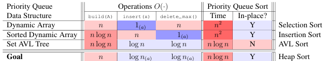
• Set AVL: O( $\lg n$ )/op $\rightarrow ^{ \text{argument} }$ O(1) find_max()
• Array: insert O(1), delete_max() O(n) (selection sort)
• Sorted Array: delete_max() O(1), insert O(n) (insertion sort)
• Heap:

Priority Queue Sort

• insert(x) for x in A (build(A))
• repeatedly delete_max() to get sorted order
• Running time is $T_{ \text{build} } + n * T_{ \text{delete\_max} } \le n * T_{ \text{insert} } + n * T_{ \text{delete\_max} }$

Complete Binary Tree

• $2^i$ nodes at depth i
• except at max depth, where nodes are left-justified
• depth order: level-order, breadth-first (for each array, there is a unique binary tree, vice versa)
• Don't need to store the tree, just store the array (implicit data structure)
• left(i) = 2i + 1, right(i) = 2i + 2, parent(i) = (i - 1) // 2

Binary Heap

• array repersenting a complete binary tree where every node satisfies the Max-Heap property at i: Q[i] $\ge$ Q[j] for node j in subtree(i)
• insert(x):

  • Q.insert_last(x)
  • max_heapify_up(|Q| - 1)
    • if Q[i] > Q[parent(i)], swap Q[i] and Q[parent(i)], then max_heapify_up(parent(i)), O( $\lg n$ )
    • else, done

• delete_max():

  • swap Q[0] and Q[|Q| - 1], remove last element (the max)
  • max_heapify_down(0)
    • if i is leaf, done
    • let j = max(left(i), right(i))
    • if Q[i] < Q[j], swap Q[i] and Q[j], then max_heapify_down(j), O( $\lg n$ )

In-place Priority Queue Sort

• Max-heap Q is a prefix of the array A, remember how many items |Q| belong to heap
• |Q| is initially zero, eventually |A| (after insertion), then zero again (after deletion)
• insert() absorbs the next item of A at index |Q| into Q
• delete_max() moves the max item of Q to the end, then abandons it by decrementing |Q|
• heapify down from the top of heap, time is $\sum \text{height} (i) =$ O(n)

Lecture 09 (Breadth-First Search)

Graph Definitions

• a collection of two things:

  • G = (V, E)
  • V = Vertices
  • E = Edges $\subseteq V \times V$
    • e = {v, w} (unordered) or (v, w) (ordered)

Simple Graph

• No self loop
• Every edge is distinct
  $|E| = O(|V|^2)$

Neighbor Sets/Adjacencies

• The outgoing neighbor set of $u \in V$ : $Adj^+ (u) = \{ v \in V | (u, v) \in E \}$
• The incoming neighbor set of $u \in V$ : $Adj^- (u) = \{ v \in V | (v, u) \in E \}$
• The out-degree of a vertex $u \in V$ : $deg^+ (u) = |Adj^+ (u)|$
• The in-degree of a vertex $u \in V$ : $deg^- (u) = |Adj^- (u)|$
• For undirected graphs, $Adj(u) = Adj^+ (u) = Adj^- (u)$ and $deg(u) = deg^+ (u) = deg^- (u)$
• Dropping superscript defaults to outgoing, i.e., $Adj(u) = Adj^+ (u)$ and $deg(u) = deg^+ (u)$
• $\sum_{v \in V} deg(v) = \begin{cases} 2|E| & \text{if undirected} \\ |E| & \text{if directed} \end{cases}$

Graph Representations

• Set maps vertex u to its neighbor set Adj(u), common to use direct access array or hash table
• store Adj(u) (need to consider directions if has) in Adjacency List, common to use array or linked list
• For common representations, Adj has size $\Theta (|V|)$, while each Adj(u) has size $\Theta (deg(u))$
• Since $\sum_{u \in V} deg(u) = O(|E|)$ , graph storable in $\Theta (|V| + |E|)$ space
• So for algorithms on graph, linear time is $\Theta (|V| + |E|)$

Path

• $p = (v_1, v_2, ..., v_k) \text{ where } (v_i, v_{i + 1}) \in E \; \forall \; i \in \{ 1,...,k-1 \}$
• length: $|p| = k - 1$ , edges in path
• simple path: a path that doesn't have the same vertex more than once

Model Graph Problems

• SINGLE_PAIR_REACHABILITY(G, s, t): Given vertices s and t, is there a path from s to t?
• SINGLE_PAIR_SHORTEST_PATH(G, s, t): Return distance from s to t and a shortest path
• SINGLE_SOURCE_SHORTEST_PATH(G, s): Return shortest distance from s to all t plus a shortest path tree

Shortest Path Tree

• For all $v \in V$ , store its parent P(v): second to last vertex on a shortest path from s
• recursively define shortest path from s to v:

  • if v = s, return [s]
  • else, return shortest path from s to P(v) + [v]

Level Set

$L_k = \{ v \in V : \delta(s,v) = k \}$

Breadth-First Search (BFS)

• Base case (i = 1): $L_0 = \{ s \} , \delta(s,s) = 0, P = \{ \}$
• Inductive Step: To compute $L_i$:

  • for every $u \in L_{i - 1}$
    • for every $v \in Adj(u)$ that does not appear in any $L_j$ for j < i:
      • add v to $L_i$ , set $\delta(s,v) = i$ , and set P(v) = u

• Repeatedly compute $L_i$ for increasing i until $L_i = \emptyset$
• Set $\delta(s,v) = \infin$ for any $v \in V$ for whitch $\delta(s,v)$ is not defined
• Running time analysis:

  • Store each $L_i$ in data structure with $\Theta(|L_i|)$ time iteration and $\Theta(1)$ time insertion
  • Checking for a vertex v in any $L_j$ for j < i can be done in $\Theta(1)$ time by checking if P(v) is defined
  • Maintain $\delta$ and P in Set data structures with $\Theta(1)$ time access (DAA or hash table)
  • Work upper bounded by $O(1) \times \sum_{u \in V} deg(u) = O(|E|)$ by handshaking lemma
  • Spend $\Theta(1)$ time per vertex to initialize and output $\delta$ and P, so total time is $O(|V| + |E|)$

Lecture 10 (Depth-First Search)

Depth-First Search (DFS)

• Straregy: Set P(s) = None and then run visit(s)

visit(u):
  for every v in Adj+(u):
    if P(v) = None:
      Set P(v) = u
      Call visit(v) 

• claim: DFS visits all reachable v $\in$ V & correctly sets P(v)
• do induction on k, distance to s

  • P(s) = s, k = 0
  • consider v with $\delta(s, v) = k+1$
  • take $u \in V$ , previous vertex on shortest path from s to v $\implies \delta(s,u) = k$
  • DFS consider $v \in Adj^+ (u)$
    • P(v) $\neq$ None
    • P(v) = None, so set P(v) = u and call visit(v)

Running Time

• Algorithm visits each vertex u at most once and spends O(1) time for each v $\in Adj^+ (u)$
• Work upper bounded by $O(1) \times \sum_{u \in V} deg^+ (u) = O(|E|)$

Graph Connectivity

• An undirected graph is connected if there is a path connecting every pair of vertices
• In a directed graph, vertex u may be reachable from v, but v may not be reachable from u
• Connectivity is more complicated for directed graphs (we won’t discuss in this class)
• Connectivity(G): is undirected graph G connected?
• Connected_Components(G): given undirected grapy G = (V, E), return partition of V into subsets $V_i \subseteq V$ (connected components) where each $V_i$ is connected in G and there are no edges between vertices from different connected components

Full-DFS and Full-BFS (to get all connected components)

• Choose an arbitrary unvisited vertex s, use BFS or DFS to explore all vertices reachable from s
• We call this algorithm Full-BFS and Full-DFS, both run in O(|V | + |E|) time

DAGS and Topological Sort

• Directed Acyclic Graph (DAG): directed graph with no directed cycles
• Topological order: Ordering f over vertices where f(u) < f(v) for all (u, v) $\in E$
• Finishing order: Order in which a full-DFS finishes visiting each vertex
• claim: if G is DAG, reverse of finishing order is a topological order
• proof: Need to prove, for every edge $(u, v) \in E$ , f(u) < f(v), Two cases:

  • If u visited before v:
    • Before visit to u finishes, will visit v (via (u, v) or otherwise)
    • Thus the visit to v finishes before visiting u
  • If v visited before u:
    • u can’t be reached from v since graph is acyclic
    • Thus the visit to v finishes before visiting u

Cycle Detection

• Full-DFS will find a topological order if a graph G = (V, E) is acyclic
• If reverse finishing order for Full-DFS is not a topological order, then G must contain a cycle
• Check if G is acyclic: for each edge (u, v), check if v is before u in reverse finishing order
• Can be done in O(|E|) time via a hash table or direct access array
• To return such a cycle, maintain the set of ancestors along the path back to s in Full-DFS
• Claim: If G contains a cycle, Full-DFS will traverse an edge from v to an ancestor of v.
• Proof: Consider a cycle $C = (v_0, v_1, ..., v_k, v_0)$

  • Without loss of generality, let $v_0$ be the first vertex in C visited by Full-DFS on the cycle
  • For each $v_i$ , before the visit to $v_i$ finishes, Full-DFS will visit $v_{i + 1}$ and finish
  • Will consider edge $(v_i, v_{i+1})$ , and if $v_{i+1}$ has not been visited, it will be visited now
  • Thus, before visit to $v_0$ finishes, Full-DFS will visit $v_k$ (for the first time, by $v_0$ assumption)
  • So, before visit to $v_0$ finishes, Full-DFS will traverse edge $(v_k, v_0)$ , where $v_0$ is an ancestor of $v_k$

Lecture 11 (Weighted Shortest Paths)

Weighted Graph

• a Weighted graph is a graph G = (V, E) together with a weight function $w: E \rightarrow Z$ (assigns each edge (u, v) $\in E$ an integer weight $w(e) = w(u, v)$ )
• (Two common ways to represent weights computationally:)

  • Inside graph representation: store edge weight with each vertex in adjacency lists
  • Store separate Set data structure mapping each edge to its weight

• We assume a representation that allows querying the weight of an edge in O(1) time

Weighted Path

• the weight $w(\pi)$ of a path $\pi = (v_1, v_2, ..., v_k)$ is the sum of the weights of its edges: $w(\pi) = \sum_{i = 1}^{k - 1} w(v_i, v_{i + 1})$
• th (weighted) shortest path from $s \in V$ to $t \in V$ is a path $\pi$ from s to t with minimum weight among all paths from s to t
• As with unweighted graphs:

  • $\delta(s, t) = \infin$ if there is no path from s to t
  • Subpaths of shortest paths are shortest paths (or else could splice in a shorter path)
  • $\delta(s, t) = inf \{ w(\pi) | \text{ path } \pi \text{ from } s \text{ to } t \}$

• Why infimum not minimum? Possible that no finite-length minimum-weight path exists

  • Can occur if there is a negative-weight cycle in the graph, then $\delta(s, t)$ would be $-\infin$

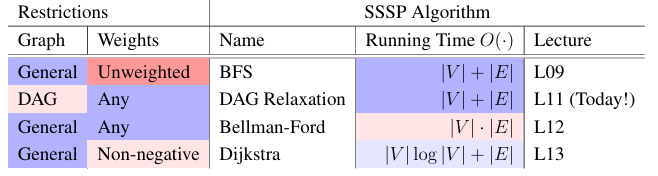
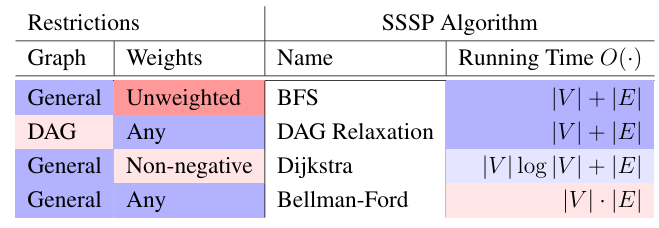
Weighted Shortest Paths Algorithms

• BFS in O(|V| + |E|) time when:

  • graph has positive weights, and all weights are the same
  • graph has positive weights, and sum of all weights at most O(|V | + |E|) (divide edge as several edges with the number of its weight, ensure linear time by using a bucket data structure to store vertices by distance)

• For general weighted graphs, we don’t know how to solve SSSP in O(|V | + |E|) time

• But if your graph is a Directed Acyclic Graph you can!

  

Shortest-Paths Tree

• (for weighted, only need P(v) fpr v with finite $\delta(s, v)$)
• Init P empty, set P(s) = None
• For each vertex $u \in V$ where $\delta (s, u)$ is finite:

  • For each $v \in Adj^+ (u)$ :
    • if $v \notin P$ and $\delta(s, u) + w(u, v) = \delta(s, v)$ , set P(v) = u

DAG Relaxation

• Maintain a distance estimate $d(s, v)$ (initially $\infin$ ) for each vertex $v \in V$ that always upper bounds the true distance $\delta(s, v)$ , then gradually improve these estimates until they equal the true distances
• When do we lower? When an edge violates the triangle inequality!

  • Triangle Inequality: the shortest-path weight from u to v cannot be greater than the shortest path from u to v through another vertex x
  • If $d(s, v) > d(s, u) + w(u, v)$ for some edge (u, v), then triangle inequality is violated

• Fix by lowering $d(s, v) \text{ to } d(s, u) + w(u, v)$ , i.e., relax (u, v) to satisfy violated constraint
• Set $d(s, v) = \infin$ for all $v \in V - \{ s \}$ , and $d(s, s) = 0$
• Process each vertex u in a topological order of G:

  • for each $v \in Adj^+ (u)$:
    • If $d(s, v) > d(s, u) + w(u, v)$:
      • relax edge $(u,v)$ , set $d(s, v) = d(s, u) + w(u, v)$

Correctness

• Claim: At end of algorithm, $d(s, v) = \delta(s, v)$ for all $v \in V$
• Proof: Induct on $k: d(s,v) = \delta(s,v)$ for all $v$ in first $k$ vertices of topological order

  • Base case: Vertex s and every vertex before s in topological order satisfies claim at start
  • Inductive step: Assume claim holds for first $k'$ vertices, let $v$ be the $(k' + 1)^{th}$ vertex
  • Consider a shortest path from s to v, and let u be the vertex preceding v on path
  • u occurs before v in topological order, so $d(s, u) = \delta(s, u)$ by inductive hypothesis
  • When we process u, we relax (u, v) if necessary, so $d(s, v) \le d(s, u) + w(u, v) = \delta(s, u) + w(u, v) = \delta(s, v)$
  • $d(s, v)$ always upper bounds $\delta(s, v)$ , since relaxation is safe, we have $d(s, v) = \delta(s, v)$

Running Time

• Initialization takes O(|V|) time
• O(|V| + |E|) time to compute topological order
• Additional work upper bounded by $O(1) \times \sum_{u \in V} deg^+ (u) = O(|E|)$
• So total time is O(|V| + |E|)

Problem Session 5

5-5 (魔方，双向BFS)

# -----------------------------------# 
# REWRITE SOLVE IMPLEMENTING PART (e) # 
# -----------------------------------# 
def solve(config): 
    # Return a sequence of moves to solve config, or None if not possible 
    def check(frontier, parent): 
        for f in frontier:
            if f in parent:
                return f
        return None

    parent_c, frontier_c = {config: None}, [config]
    parent_s, frontier_s = {SOLVED: None}, [SOLVED]
    middle = check(frontier_c, parent_s)
    while middle is None:
        frontier_c = explore_frontier(frontier_c, parent_c)
        middle = check(frontier_c, parent_s)
        if middle: break
        frontier_s = explore_frontier(frontier_s, parent_s)
        middle = check(frontier_s, parent_c)
    if middle:
        path_c = path_to_config(middle, parent_c)
        path_s = path_to_config(middle, parent_s)
        path_s.pop()
        path_s.reverse()
        return moves_from_path(path_c + path_s) 
    return None
      
# ---------------------------------------# 
# READ, BUT DO NOT MODIFY CODE BELOW HERE # 
# ---------------------------------------# 
# Pocket Cube configurations are represented by length 24 strings 
# Each character repesents the color of a small cube face 
# Faces are layed out in reading order of a Latin cross unfolding of the cube 

SOLVED = '000011223344112233445555'
def config_str(config): 
    # Return config string representation as a Latin cross unfolding 
    return """ 
            %s%s 
            %s%s 
        %s%s%s%s%s%s%s%s 
        %s%s%s%s%s%s%s%s 
            %s%s 
            %s%s 
    """ % tuple(config) 

def shift(A, d, ps): 
    # Circularly shift values at indices ps in list A by d positions 
    values = [A[p] for p in ps] 
    k = len(ps) 
    for i in range(k): 
        A[ps[i]] = values[(i -d) % k] 

def rotate(config, face, sgn): 
    # Returns new config by rotating input face of input config 
    # Rotation is clockwise if sgn == 1, counterclockwise if sgn == -1 
    assert face in (0, 1, 2) 
    assert sgn in (-1, 1) 
    if face is None: return config 
    new_config = list(config) 
    if face == 0: 
        shift(new_config, 1*sgn, [0,1,3,2]) 
        shift(new_config, 2*sgn, [11,10,9,8,7,6,5,4])
    elif face == 1: 
        shift(new_config, 1*sgn, [4,5,13,12]) 
        shift(new_config, 2*sgn, [0,2,6,14,20,22,19,11]) 
    elif face == 2: 
        shift(new_config, 1*sgn, [6,7,15,14]) 
        shift(new_config, 2*sgn, [2,3,8,16,21,20,13,5]) 
    return ''.join(new_config) 

def neighbors(config): 
    # Return neighbors of config 
    ns = [] 
    for face in (0, 1, 2): 
        for sgn in (-1, 1): 
            ns.append(rotate(config, face, sgn)) 
    return ns 

def explore_frontier(frontier, parent, verbose = False): 
    # Explore frontier, adding new configs to parent and new_frontier 
    # Prints size of frontier if verbose is True 
    if verbose: 
        print('Exploring next frontier containing # configs: %s' % len(frontier)) 
    new_frontier = [] 
    for f in frontier: 
        for config in neighbors(f): 
            if config not in parent: 
                parent[config] = f 
                new_frontier.append(config) 
    return new_frontier 

def path_to_config(config, parent): 
    # Return path of configurations from root of parent tree to config 
    path = [config] 
    while path[-1] is not None: 
        path.append(parent[path[-1]]) 
    path.pop() 
    path.reverse() 
    return path 

def moves_from_path(path): 
    # Given path of configurations, return list of moves relating them 
     # Returns None if any adjacent configs on path are not related by a move 
    moves = [] 
    for i in range(1, len(path)): 
        move = None 
        for face in (0, 1, 2): 
            for sgn in (-1, 1): 
                if rotate(path[i -1], face, sgn) == path[i]: 
                    move = (face, sgn) 
                    moves.append(move) 
        if move is None: 
            return None 
    return moves 

def path_from_moves(config, moves): 
    # Return the path of configurations from input config applying input moves 
    path = [config] 
    for move in moves: 
        face, sgn = move 
        config = rotate(config, face, sgn) 
        path.append(config) 
    return path 

def scramble(config, n): 
    # Returns new configuration by appling n random moves to config 
    from random import randint 
    for _ in range(n): 
        ns = neighbors(config) 
        i = randint(0, 2) 
        config = ns[i] 
    return config 

def check(config, moves, verbose = False): 
    # Checks whether applying moves to config results in the solved config 
    if verbose: 
        print('Making %s moves from starting configuration:' % len(moves)) 
    path = path_from_moves(config, moves) 
    if verbose: 
        print(config_str(config)) 
    for i in range(1, len(path)): 
        face, sgn = moves[i -1] 
        direction = 'clockwise' 
        if sgn == -1: 
         direction = 'counterclockwise' 
        if verbose: 
            print('Rotating face %s %s:' % (face, direction)) 
            print(config_str(path[i])) 
    return path[-1] == SOLVED 

def test(config): 
    print('Solving configuration:') 
    print(config_str(config)) 
    moves = solve(config) 
    if moves is None: 
        print('Path to solved state not found... :(') 
        return 
    print('Path to solved state found!') 
    if check(config, moves): 
        print('Move sequence terminated at solved state!') 
    else: 
        print('Move sequence did not terminate at solved state... :(') 

if __name__ == '__main__': 
  config = scramble(SOLVED, 100) 
  test(config)

Lecture 12 (Bellman-Ford)

• Goal: SSSP for a graph with negative weights

  • Conpute $\delta(s, v)$ for all $v \in V$ ( $-\infin$ if v reachable from a negative-weight cycle)
  • if a negative-weight cycle is reachable from s, return one such cycle

Warmups

Exercise 1

Given undirected graph G, return whether G contains a negative-weight cycle

Solution: Return Yes if there is an edge with negative weight in G in O(|E|) time

Exercise 2

Given SSSP algorithm A that runs in O(|V|(|V| + |E|)) time,
show how to use it to solve SSSP in O(|V||E|) time

Solution: Run BFS or DFS to find the vertices reachable from s in O(|E|) time

• Mark each vertex v not reachable from s with $\delta(s, v) = \infin$ in O(|V|) time
• Make graph G' = (V', E') with only vertices reachable from s in O(|V| + |E|) time
• Run A from s in G'
• G' is connected, so |V'| = O(|E'|) = O(|E|), so A runs in O(|V||E|) time

Simple Shortest Paths

• Claim 1: If $\delta(s,v)$ is finite, $\exist$ a shortest path from s to v thai is simple, simple path have at most |V| - 1 edges

  proof: consider if this claim is false, then every shortest path from s to v has a cycle, then the weight of the cycle can't be negative, so we can remove the cycle to get a shorter path, contradiction

Negative Cycle Witness

• Idea: find shortest path by limit the number of edges in the path, k-Edge distance $\delta_k (s,v)$ : the minimum weight of any path from s to v using $\le$ k edges

• Idea: Compute $\delta_{|V| - 1} (s,v)$ and $\delta_{|V|} (s,v)$ for all $v \in V$

  • If $\delta(s,v) \neq - \infin$ , $\delta(s,v) = \delta_{|V|-1} (s,v)$ , since a shortest path is simple (or nonexistent)
  • If $\delta_{|V|} (s,v) < \delta_{|V| - 1} (s,v)$
    • there exists a shorter non-simple path to v, so $\delta_{|V|}(s,v) = - \infin$
    • call v a (negative cycle) witness
  • However, there may be vertices with $-\infin$ shortest-path weight that are not witnesses

• Claim 2: If $\delta(s,v) = -\infin$ , then v is reachable from a witnesses

  proof: Suffices to prove: every negative-weight cycle reachable from s contains a witness

  • Consider a negative-weight cycle C reachable from s
  • For $v \in C$ denotes $v$ 's predecessor in C, where $\sum_{v \in C} w(v', v) <0$
  • Then $\delta_{|V|}(s,v) \le \delta_{|V| - 1}(s,v') + w(v', v)$ (RHS weight of some path on ≤ |V | vertices)
  • So $\sum_{v \in C} \delta_{|V|}(s,v) \le \sum_{v \in C} \delta_{|V| - 1}(s,v') +\sum_{v \in C} w(v', v) < \sum_{v \in C} \delta_{|V| - 1}(s,v)$ (C is negative cycle, so the sum is negative)
  • If C contains no witness, $\delta_{|V|}(s,v) \ge \delta_{|V| -1}(s,v)$ for all $v \in C$ , a contradiction

Bellman-Ford

• Idea: Use graph duplication: make multiple copies (or levels) of the graph

• |V| + 1 levels: vertex $v_k$ in level k represents reaching vertex v from s using ≤ k edges

• If we connect edges from one level to only higher levels, resulting graph is a DAG!

  ---

• Construct new DAG G' = (V', E') from G = (V, E):

  • G' has |V|(|V| + 1) vertices: $V' = \{ v_k | v \in V, k = 0, 1, ..., |V| \}$
  • G' has |V|(|V| + |E|) edges:
    • |V| edges $( v_{k-1} , v_k )$ for $k \in \{ 1, ..., |V| \}$ and $v \in V$ with weight 0 (stay at v)
    • |V| edges $( v_{k-1} , v_k )$ for $k \in \{ 1, ..., |V| \}$ of weight $w(u,v)$ for each $(u,v) \in E$

• Run DAG Relaxation on G' from $S_0$ to compute $\delta(s_0, v_k)$ for all $v_k \in V'$

• For each vertex: set $d(s,v) = \delta(s_0, v_{|V| - 1})$

• For each witness $u \in V$ where $\delta(s_0, u_{|V|}) < \delta(s_0, u_{|V| -1})$ :

  • For each vertex v reachable from u in G:
    • set $d(s,v) = -\infin$

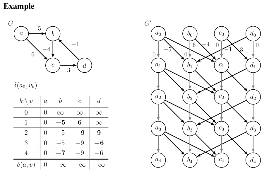
Correctness

• Claim 3: $\delta(s_0, v_k) = \delta_k (s,v)$ for all $v \in V$ and $k \in \{ 0, 1, ..., |V| \}$

  proof: By induction on k:

  • Base case: true for all $v \in V$ when k = 0 (only $v_0$ reachable from $s_0$ is v = s)
  • Inductive Step: Assume true for all k < k', prove for k = k'

  • $\begin{aligned} \delta(s_0, v_{k'}) = \min \{ & \delta(s_0, u_{k'-1}) + w(u_{k'-1},v_{k'}) \; | \; u_{k'-1} \in Adj^- (v_{k'}) \} \\ = \min \{ \{ & \delta(s_0, u_{k'-1}) + w(u,v) \; | \; u \in Adj^-(v) \} \cup \{ \delta(s_0, v_{k'-1}) \} \\ = \min \{ \{ & \delta_{k'-1}(s_0, u) + w(u,v) \; | \; u \in Adj^-(v) \} \cup \{ \delta_{k'-1}(s, v) \} \text{ (by induction)} \\ = & \delta_{k'}(s,v) \end{aligned}$

• Claim 4: At the end of Bellman-Ford $d(s,v) = \delta(s,v)$

  proof: Correctly computes $\delta_{|V| - 1}(s,v)$ and $\delta_{|V|}(s,v)$ for all $v \in V$ by Claim 3

  • If $\delta(s,v) \neq -\infin$ , then correctly sets $d(s,v) = \delta(s,v) = \delta_{|V| - 1}(s,v)$ by Claim 1
  • Then sets $d(s,v) = -\infin$ for all v reachable from a witness by Claim 2

Running Time

• G' has size O(|V|(|V| + |E|)) and can be constructed in as much time
• Running DAG Relaxation on G' takes linear time in the size of G'
• Does O(1) work for each vertex reachable from a witness
• Finding reachability of a witness takes O(|E|) time, with at most O(|V|) witnesses: O(|V||E|)
• (Alternatively, connect super node x to witnesses via 0-weight edges, linear search from x)
• Pruning G at start to only subgraph reachable from s yields O(|V||E|)-time algorithm

Extras: Return Negative-Weight Cycle or Space Optimization

• Claim 5: Shortest $s_0 - v_{|V|}$ path $\pi$ for any witness v contains a negative-weight cycle in G

  proof: Since $\pi$ contains $|V|+1$ edges, must contain at least one cycle C in G

  • C has negative weight (otherwise, remove C to make path $\pi'$ with fewer vertices and $w(\pi') \le w(\pi)$ , contradicting witness v)

• Can use just O(|V|) space by storing only $\delta(s_0, v_{k-1})$ and $\delta(s_0, v_k)$ for each k from 1 to |V|
• Traditionally, Bellman-Ford stores only one value per vertex, attempting to relax every edge
  in |V| rounds; but estimates do not correspond to k-Edge Distances, so analysis trickier
• But these space optimizations don’t return a negative weight cycle

Lecture 13 (Dijkstra’s Algorithm)

• Today: faster for general graphs with non-negative edge weights

Non-negative Edge Weights

• Idea: Generalize BFS approach to weighted graphs:

  • Grow a sphere centered at source s
  • Repeatedly explore closer vertices before further ones
  • But how to explore closer vertices if you don’t know distances beforehand?

• Observation 1: If weights non-negative, monotonic distance increase along shortest paths

  • if vertex u is on a shortest path from s to v, then $\delta(s,u) \le \delta(s,v)$
  • Let $V_x \subset V$ be the subset of vertices reachable within distance $\le x$ from s
  • If u $\in V_x$ , then any shortest path from s to v only contains vertices from $V_x$
  • Perhaps grow %V_x$ one vertex at a time! (but growing for every x is slow if weights large)

• Observation 2: Can solve SSSP fast if given order of vertices in increasing distance from s

  • Remove edges that go against this order (since cannot participate in shortest paths)
  • May still have cycles if zero-weight edges: repeatedly collapse into single vertices
  • Compute $\delta(s,v)$ for each $v \in V$ using DAG relaxation in O(|V | + |E|) time

Dijkstra's Algorithm

• Idea: Relax edges from each vertex in increasing order of distance from source s
• Idea: Efficiently find next vertex in the order using a data structure

Changeable Priority Queue

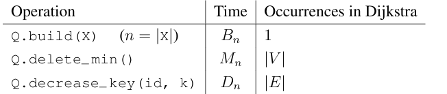
• Q on items with keys and unique IDs, supporting operations:

• Q.build(X): initialize Q with items in iterator X
• Q.delete_min(): remove an item with minimum key
• Q.decrease_key(id, k): find stored item with ID id and change key to a smaller key k

• Implement: cross-linking a Priority Queue Q' and a Dictionary D mapping IDs into Q'

• Assume vertex IDs are integers from 0 to |V| - 1 so can use a direct access array for D

• For brevity, say item x is the tuple (x.id, x.key)

  ---

Steps

• Set $d(s, v) = \infin$ for all $v \in V$ , then set $d(s, s) = 0$
• Build changeable priority queue Q with an item (v, d(s, v)) for each vertex $v \in V$
• While Q not empty, delete an item (u, d(s, u)) from Q that has minimum $d(s,u)$
  • For vertex v in outgoing adjacencies $Adj^+(u)$ :
    • If $d(s,v) > d(s,u) + w(u,v)$ :
      • Relax edge $(u,v)$ , set $d(s,v) = d(s,u) + w(u,v)$
      • decrease key of item with ID v in Q to $d(s,v)$

Correctness

• Claim: At end of Dijkstra’s algorithm, $d(s,v) = \delta(s,v)$ for all $v \in V$
• Proof:

  • If relaxation sets $d(s,v)$ to $\delta(s,v)$ , then $d(s,v) = \delta(s,v)$ at the end of the algorithm
    • Relaxation can only decrease estimates $d(s,v)$
    • Relaxation is safe, i.e., maintains that each $d(s,v)$ is weight of a path to $v$ (or $\infin$ )
  • Suffices to show $d(s,v) = \delta(s,v)$ when vertex v is removed from Q
    • Proof by induction on first k vertices removed from Q
    • Base Case (k =1): s is first vertex removed from Q, and $d(s,s) = \delta(s,s) = 0$
    • Inductive Step: Assume true for k < k', consider k'th vertex v' removed from Q
    • Consider some shortest path $\pi$ from s to v', with $w(\pi) = \delta(s,v')$
    • Let (x, y) be the first edge in $\pi$ where y is not among first k' - 1 (perhaps y = v')
    • When x was removed from Q, by inductive hypothesis, $d(s,x) = \delta(s,x)$
      • So: $d(s,y) \le d(s,x) + w(x,y)$ relaxed edge (x, y) when removed x
      • $= \delta(s,x) + w(x,y) = \delta(s,y)$ subpaths of shortest paths are shortest paths
      • $\le \delta(s,v')$ non-negative edge weights
      • $\le d(s,v')$ relaxation is safe
      • $\le d(s,y)$ assume that v' is vertex with minimum d(s, v') in Q, but y is still in Q, so $d(s,v') \le d(s,y)$
    • So $d(s,v') = \delta(s,v')$ , as desired

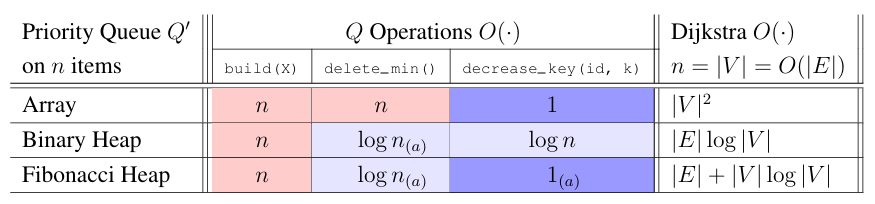
Running Time

• Count operations on changeable priority queue Q, assuming it contains n items:
  

• Total running time is $O(B_{|V|} + |V| * M_{|V|} + |E| * D_{|V|})$

• Assume pruned graph to search only vertices reachable from the source, so |V| = O(|E|)
  

• If graph is dense, i.e., |E| = $\Theta(|V|^2)$ , then array-based priority queue is best, and Dijkstra’s runs in $O(|V|^2)$ time

• If graph is sparse, i.e., |E| = O(|V|) , then binary-heap-based priority queue is best, and Dijkstra’s runs in O((|V| + |E|) log |V|) = O(|E| log |V|) time

• A Fibonacci Heap is theoretically good in all cases, but is not used much in practice

• We won’t discuss Fibonacci Heaps in 6.006 (see 6.854 or CLRS chapter 19 for details)

• You should assume Dijkstra runs in O(|E|+|V| log|V|) time when using in theory problems

Summary: Weighted Single-Source Shortest Paths

• Doing a SSSP algorithm |V| times is actually pretty good, since output has size $O(|V|^2)$
• Can do better than |V| · O(|V| · |E|) for general graphs with negative weights (next time!)

Lecture 14 (Dijkstra’s Algorithm)

All-Pairs Shortest Paths (APSP)

• Input: directed graph G = (V, E) with weights $w: E \rightarrow \mathbb{Z}$
• Output: $\delta(u,v)$ for $\forall u,v \in V$ , or abort if G contains a negative-weight cycle
• Useful when understanding whole network, e.g., transportation, circuit layout, supply chains...
• Just doing a SSSP algorithm |V| times is actually pretty good, since output has size $O(|V|^2)$
  • $|V|·O(|V|+|E|)$ with BFS if weights positive and bounded by $O(|V| + |E|)$
  • $|V|·O(|V|+|E|)$ with DAG Relaxation if acyclic
  • $|V|·O(|V| \log |V|+|E|)$ with Dijkstra if weights non-negative or graph undirected
  • $|V|·O(|V|·|E|)$ with Bellman-Ford (general)
• Today: Solve APSP in any weighted graph in $|V|·O(|V| \log |V|+|E|)$ time

Approach

• Idea: Make all edge weights non-negative while preserving shortest paths
• i.e., reweight G to G' with no negative weights, where a shortest path in G is shortest in G'
• If non-negative, then just run Dijkstra |V| times to solve APSP
• Claim: Can compute distances in G from distances in G' in O(|V|(|V| + |E|)) time
  • Compute shortest-path tree from distances, for each $s \in V$ in O(|V| + |E|) time (Lec11)
  • Also shortest-paths tree in G, so traverse tree with DFS while also computing distances
  • Takes O(|V| · (|V| + |E|)) time (which is less time than |V| times Dijkstra)
• Claim: This method is not possible if G contains a negative-weight cycle
• Proof: Shortest paths are simple if no negative weights, but are not simple if have negative-weight cycle
• Given graph G with negative weights but no negative-weight cycles, can we make edge weights non-negative while preserving shortest paths?

Making Weights Non-negative 1

• Idea: Given vertex v, add h to all outgoing edges and subtract h from all incoming edges
• Claim: Shortest paths are preserved under the above reweighting
• Proof:

  • Weight of every path starting at v changes by h
  • Weight of every path ending at v changes by −h
  • Weight of a path passing through v does not change (locally)

• This is a very general and useful trick to transform a graph while preserving shortest paths! Even works with multiple vertices!
• Define a potential function $h: V \rightarrow \mathbb{Z}$ mapping each vertex $v \in V$ to a potential $h(v)$
• Make graph G': same as G but edge $(u,v) \in E$ has weight $w'(u,v) = w(u,v) + h(u) - h(v)$
• Claim: Shortest paths in G are also shortest paths in G'
• Proof:

  • Weight of path $\pi = (v_0, v_1, ..., v_k)$ in G is $w(\pi) = \sum^k_{i = 1} w(v_{i-1} , v_i )$
  • Weight of $\pi$ in G' is $\sum^k_{i = 1} w(v_{i-1} , v_i ) + h(v_{i-1}) - h(v_i) = w(\pi) + h(v_0) - h(v_k)$
  • (Sum of h’s telescope, since there is a positive and negative $h(v_i)$ for each interior i)
  • Every path from $v_0$ to $v_k$ changes weight by the same amount $h(v_0) - h(v_k)$ , so shortest paths preserved

Making Weights Non-negative 2

• Can we find a potential function such that G' has no negative edge weights? i.e., is there an h such that $w'(u,v) = w(u,v) + h(u) - h(v) \ge 0$ for all $(u,v) \in E$ ?
• Rearranging, we want $h(v) \le w(u,v) + h(u)$ ( $\delta(v) \le w(u,v) + \delta(u)$ ) for all $(u,v) \in E$ , looks like triangle inequality
• Idea (x): Condition would be satisfied if $h(v) = \delta(s,v)$ and $\delta(s,v)$ is finite for some s, But graph may be disconnected, so may not exist any such vertex s...
• Idea: Add a new super vertex s with a directed 0-weight edge to every $v \in V$ , then let $h(v) = \delta(s,v)$
• $\delta(s,v) \le 0$ for all $v \in V$ , since can reach v from s with a 0-weight edge
• Claim: If $\delta(s,v) = - \infin$ for any $v \in V$ , then the original graph has a negative-weight cycle
• Proof:

  • Adding s does not introduce new cycles (s has no incoming edges)
  • So if reweighted graph has a negative-weight cycle, so does the original graph

• Alternatively, if $\delta(s,v)$ is finite for all $v \in V$
  • $w'(u,v) = w(u,v) + h(u) - h(v) \ge 0$ for every $(u,v) \in E$ by triangle inequality
  • New weights in G' are non-negative while preserving shortest paths!

Johnson’s Algorithm

• Construct $G_x$ from G by adding new vertex s with 0-weight edges to all $v \in V$
• Compute $\delta_x(x,v)$ for every $v \in V_x$ using Bellman-Ford
• If $\delta_x(x,v) = - \infin$ for any $v \in V_x$
  • Abort (since there is a negative-weight cycle in G)
• Else:
  • Reweight each edge $w'(u,v) = w(u,v) + \delta_x(x,u) - \delta_x(x,v)$ to form graph G'
  • For each $u \in V$:
    • Compute shortest-path distances $\delta'(u,v)$ for all $v \in V$ in G' using Dijkstra
    • For each $v \in V$ , compute $\delta(u,v) = \delta'(u,v) - \delta_x(x,u) + \delta_x(x,v)$

Correctness

• Already proved that transformation from G to G' preserves shortest paths
• Rest reduces to correctness of Bellman-Ford and Dijkstra
• Reducing from Signed APSP to Non-negative APSP
• Reductions save time! No induction today!

Running Time

• O(|V| + |E|) time to construct $G_x$
• O(|V| · |E|) time to run Bellman-Ford on $G_x$
• O(|V| + |E|) time to construct G'
• O(|V| · (|V| log |V| + |E|)) time to run Dijkstra |V| times on G'
• $O(|V|^2)$ time to compute distances in G from distances in G'
• $O(|V|^2 \log |V| + |V|·|E|)$ total time

Problem Session 7

7-5 Shipping Servers

The video streaming service UsTube has decided to relocate across country, and needs to ship their servers by truck from San Francisco, CA to Cambridge, MA. They will pay third-party trucking companies to transport servers from city to city. An intern at UsTube has compiled a list R of all n available trucking routes; each available route $r_i \in R$ is a tuple $(s_i, t_i, w_i, c_i)$ , where $s_i$ and $t_i$ are respectively the names of the starting and ending cities of the trucking route, $w_i$ is the positive integer weight capacity of the truck, and $c_i$ is the positive integer cost of shipping along that route (cost is the same for shipping any weight from 0 to $w_i$ ). Note that the existence of a shipping route from $s_i$ to $t_i$ does not imply a shipping route from $t_i$ to $s_i$ . Some of UsTube’s servers are too heavy to fit on any truck, so they will need to transfer them to smaller servers for the move. Assume that it is possible to ship some finite weight from San Francisco to Cambridge via some routes in R. Help UsTube evaluate their shipping options.

• Assuming that the number of cities appearing in any of the n trucking routes is less than $3 \sqrt{n}$ , describe an O(n)-time algorithm to return both: (1) the weight $w^*$ of the largest single server
  that can be shipped from San Francisco to Cambridge via a sequence of trucking routes, and (2) the minimum cost to ship such a server with weight $w^*$ .

Solution:

• Step 1: Minimum Cost for a Given Weight
  • Suppose we know a candidate server weight $w^*$. We can construct a graph $G_c = (V_c, E_c)$ as follows:
  • Each city corresponds to a vertex in $V_c$.
  • For each trucking route $(s_i, t_i, w_i, c_i)$ such that $w_i \ge w^*$, add a directed edge from $s_i$ to $t_i$ with weight $c_i$.
  • Then, running Dijkstra's algorithm from the vertex corresponding to San Francisco allows us to compute the minimum cost to ship a server of weight $w^*$ to Cambridge.
  • Since the number of vertices is $O(n)$ and the number of edges is $O(n\sqrt{n})$ (per the problem assumptions), Dijkstra runs in $O(n)$ time if a direct-access array or hash table is used for the priority queue.
• Step 2: Finding the Maximum Shippable Weight $w^*$
  • We construct a graph $G_w = (V_w, E_w)$ similar to $G_c$, but the edge weights represent capacities instead of costs:
    • Each city corresponds to a vertex in $V_w$.
    • For every trucking route $(s_i, t_i, w_i, c_i)$, add a directed edge from $s_i$ to $t_i$ with weight $w_i$.
    • Let $s$ and $t$ denote the vertices corresponding to San Francisco and Cambridge, respectively.
• Step 3: Modified Dijkstra for Bottleneck Paths
  • We can modify Dijkstra's algorithm to compute the maximum bottleneck instead of the shortest path:
  1. Initialization:
     • Set the bottleneck estimate $b_s(v) = 0$ for all vertices $v$, representing no shipment.
     • Set $b_s(s) = +\infty$, as there is no limit at the starting vertex.
  2. Priority Queue:
     • Insert all vertices into a max-priority queue based on their current bottleneck estimates.
  3. Relaxation:
     • Repeatedly remove the vertex $u$ with the largest bottleneck estimate.
     • For each outgoing edge $(u, v)$ with weight $w_i$, update:
       $b_s(v) = \max(\min(b_s(u), w_i),\ b_s(v))$
     • This ensures that $b_s(v)$ always reflects the maximum bottleneck of any path discovered to $v$.
  4. Termination:
     • When all vertices are removed from the queue, $b_s(t)$ gives the maximum shippable weight $w^*$.
• Step 4: Correctness and Complexity
  • The correctness of this modified Dijkstra follows the same logic as the standard Dijkstra algorithm: when a vertex $v$ is removed from the queue, $b_s(v)$ equals the maximum bottleneck $b(s,v)$.
  • Once we know $w^* = b_s(t)$, we can apply Step 1 to compute the minimum shipping cost for a server of weight $w^*$.
  • Since the modification only changes the relaxation step from one constant-time operation to another, and the graph has $O(n)$ vertices and $O(n\sqrt{n})$ edges, the algorithm runs in $O(n)$ time with an appropriate priority queue.

Lecture 15 (Dynamic Programming I, SRTBOT, Fib, DAGs, Bowling)

• SRTBOT: recursive problem solving framework
• DP: recursion + memoization

How to solve a problem recursively (SRT BOT)

• 1. Subproblem definition
  • Describe the meaning of a subproblem in words, in terms of parameters
  • Often subsets of input: prefixes, suffixes, contiguous substrings of a sequence
  • Often record partial state: add subproblems by incrementing some auxiliary variables
• 2. Relate subproblem solutions recursively
  • $x(i) = f(x(j) \; ...)$ for one and more subproblems $j < i$
• 3. Topological order on subproblems (⇒ subproblem DAG)
• 4. Base cases of relation
  • State solutions for all (reachable) independent subproblems where relation breaks down
• 5. Original problem solution via subproblem(s)
  • Show how to compute solution to original problem from solutions to subproblem(s)
  • Possibly use parent pointers to recover actual solution, not just objective function
• 6. Time analysis
  • $\sum_{x \in X} \text{work} (x)$ , or if $\text{work} (x) = O(W)$ for all $x \in X$ , then $O(|X|·W)$
  • $\text{work} (x)$ measures nonrecursive work in relation; treat recursions as taking $O(1)$ time

Fibonacci Numbers

• subproblem: compute $F(n)$ , the n’th Fibonacci number
• relation: $F(n) = F(n - 1) + F(n - 2)$ for $n \ge 2$
• topological order: increasing n
• base cases: $F(0) = 0$ , $F(1) = 1$
• original problem solution: $F(N)$
  • Divide and conquer implies a tree of recursive calls (draw tree)
• time analysis: $T(n) = T(n - 1) + T(n - 2) + O(1) > 2T(n - 2)$ ⇒ $T(n) = \Omega (2^ {n / 2} )$ exponential...

• There is a problem with naive recursion: Subproblem $F(k)$ solved multiple times ( $F(n - k)$ times)
• avoid this with memoization: store subproblem solutions in a table when first computed, reuse later

Re-using Subproblem Solutions

• Draw subproblem dependencies as a DAG
• To solve, either:
  • Top down: record subproblem solutions in a memo and re-use (recursion + memoization)
  • Bottom up: solve subproblems in topological sort order (usually via loops)

# recursive solution (top down)
def fib(n): 
  memo = {} 
  def F(i):
    if i < 2: return i
    if i not in memo:
      memo[i] = F(i - 1) + F(i - 2)
    return memo[i]
  return F(n)

# iterative solution (bottom up) 
def fib(n): 
  F = {} 
  F[0], F[1] = 0, 1
  for i in range(2, n + 1): 
    F[i] = F[i - 1] + F[i - 2]
  return F[n]

• A subtlety is that Fibonacci numbers grow to $\Theta(n)$ bits long, potentially $\gg$ word size w
• Each addition costs $O(\lceil n/w \rceil)$ time (in w-bits RAM model, since adding two b-bit numbers takes O(⌈b/w⌉) time, and $F(n)$ grows to $\Theta(n)$ bits)
• So total cost is $O(n * \lceil n/w \rceil) = O(n + n^2 / w)$ time

Dynamic Programming

• Existence of recursive solution implies decomposable subproblems
• Recursive algorithm implies a graph of computation
• Dynamic programming if subproblem dependencies overlap (DAG, in-degree > 1)
• “Recurse but re-use” (Top down: record and lookup subproblem solutions)
• “Careful brute force” (Bottom up: do each subproblem in order)
• Often useful for counting/optimization problems: almost trivially correct recurrences

DAG Shortest Paths

• Recall the DAG SSSP problem: given a DAG G and vertex s, compute $\delta (s,v)$ for all $v \in V$
• subproblem: compute $\delta (s,v)$ for each $v \in V$
• relation: $\delta (s,v) = \min_{u \in Adj^- (v)} \{ \delta (s,u) + w(u,v) \}$ for all $v \neq s$
• topological order: any topological sort of G
• base case: $\delta (s,s) = 0$
• original problem solution: $\delta (s,v)$ for all $v \in V$
• time analysis: $\sum _{v \in V} (1 + | Adj^- (v)|) = O(|V| + |E|)$ time (each subproblem solved once, each edge examined once)
• DAG Relaxation computes the same min values as this dynamic program, just
  • step-by-step (if new value < min, update min via edge relaxation), and
  • from the perspective of $u$ and $Adj^+ (u)$ instead of $v$ and $Adj^- (v)$

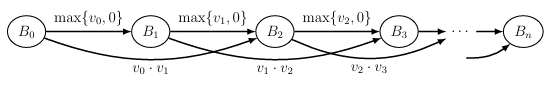
Bowling

• Given n pins labeled 0, 1,...,n − 1
• Pin i has value $v_i$
• Ball of size similar to pin can hit either
  • 1 pin i, in which case we get $v_i$ points
  • 2 adjacent pins i and i + 1, in which case we get $v_i · v_{i + 1}$ points
• Once a pin is hit, it can’t be hit again (removed)
• Problem: Throw zero or more balls to maximize total points

Bowling Algorithms

Dynamic programming algorithm: use suffixes

• subproblem: $B(i)$ = maximum score starting with just pins i, i + 1,..., n − 1, for $i = 0 \le i \le n$
• relation:
  • Locally brute-force what could happen with first pin (original pin i):
    skip pin, hit one pin, hit two pins
  • Reduce to smaller suffix and recurse, either $B(i + 1)$ or $B(i + 2)$
  • $B(i) = \max \{ B(i + 1), B(i + 1) + v_i , B(i + 2) + v_i · v_{i + 1} \}$ for $0 \le i \le n - 2$
• topological order: decreasing i
• base cases: $B(n) = B(n + 1) = 0$ , $B(n - 1) = v_{n - 1}$
• original problem solution: $B(0)$
• time analysis: O(n) subproblems, O(1) work each ⇒ O(n) time

Equivalent to maximum-weight path in Subproblem DAG:

# recursive solution (top down)
def bowl(v):
  memo = {} 
  def B(i): 
    if i >= len(v): return 0 
    if i not in memo: 
      memo[i] = max(B(i+1), 
                    v[i] + B(i+1), 
                    v[i] * v[i+1] + B(i+2))
    return memo[i]
  return B(0)

# iterative solution (bottom up) 
def bowl(v): 
  B = {} 
  B[len(v)] = 0
  B[len(v) + 1] = 0
  for i in reversed(range(len(v))): 
      B[i] = max(B[i + 1], 
                 v[i] + B[i + 1], 
                 v[i] * v[i + 1] + B[i + 2])
  return B[0]

Lecture 16 (Dynamic Programming II, LCS, LIS, Coins)

Dynamic Programming step(SRT BOT)

1. Subproblem definition $\;\;\;$ subproblem $x \in X$
   • Describe the meaning of a subproblem in words, in terms of parameters
   • Often subsets of input: prefixes, suffixes, contiguous substrings of a sequence
   • Ofen multiple possible subsets across multiple parameters
   • Often record partial state: add subproblems by incrementing some auxiliary variables
2. Relate subproblem solutions recursively $\;\;\;$ $x(i) = f(x(j) \; ...)$ for one and more subproblems $j < i$
   • Identify a question about a subproblem solution that, if you knew the answer to, reduces the subproblem to smaller subproblem(s)
   • Locally brute-force all possible answers to the question
3. Topological order to argue relation is acyclic and subproblems for a DAG (⇒ subproblem DAG)
4. Base cases
   • State solutions for all (reachable) independent subproblems where relation breaks down
5. Original problem
   • Show how to compute solution to original problem from solutions to subproblem(s)
   • Possibly use parent pointers to recover actual solution, not just objective function
6. Time analysis
   • $\sum_{x \in X} \text{work} (x)$ , or if $\text{work} (x) = O(W)$ for all $x \in X$ , then $|X|·O(W)$
   • $\text{work} (x)$ measures nonrecursive work in relation; treat recursions as taking $O(1)$ time

Longest Common Subsequence (LCS)

• Given two strings A and B, find the longest string that is a subsequence of both A and B
• Subproblems:
  • $x(i,j)$ = length of longest common subsequence of A[i:] and B[j:]. ( $0 \le i \le |A| , 0 \le j \le |B|$ )
• Relate:
  • $x(i, j) = \begin{cases} x(i + 1, j + 1) + 1 & \text{if } A[i] = B[j] \\ \max\{x(i + 1, j), x(i, j + 1)\} & \text{otherwise} \end{cases}$
• Topological order:
  • subproblem $x(i,j)$ depend only on strictly larger i or j, so order by decreasing i + j.
  • Nice order for bottom-up code: Decreasing i, then decreasing j
• Base:
  • $x(|A|, j) = x(i, |B|) = 0$ (one string is empty)
• Original problem:
  • length of LCS is $x(0,0)$ , can recover LCS with parent pointers
• Time:
  • subproblems: (|A| + 1)(|B| + 1) = O(|A|·|B|)

def lcs(A, B): 
  a, b = len(A), len(B) 
  x = [[0] * (b + 1) for _ in range(a + 1)] 
  for i in reversed(range(a)): 
    for j in reversed(range(b)): 
      if A[i] == B[j]: 
        x[i][j] = x[i + 1][j + 1] + 1 
      else: 
        x[i][j] = max(x[i + 1][j], x[i][j 
  return x[0][0]

Longest increasing Subsequence (LIS)

• Given array A of n numbers, find length of longest increasing subsequence
• Subproblems:
  • $x(i)$ = length of longest increasing subsequence of A[i:] ( $0 \le i \le |A|$ )
• Relate:
  • $x(i) = \max \{1 + x(j) \; | \; j > i \text{ and } A[j] > A[i]\} \cup \{1\}$
• Topological order:
  • Decreasing i
• Base (no base)
• Original problem:
  • length of LIS is $\max_{0 \le i < |A|} x(i)$ , can recover LIS with parent pointers
• Time:
  • subproblems: |A| = n
  • work per subproblem: O(n) to check all j > i
  • total time: O(n^2)

Alternating Coin Game

Solution 1 : (exploits that this is a zero-sum game: I take all coins you don't)

• Given sequence of n coins with values $v_0, v_1,...,v_{n-1}$ . Tow players, each take turns choosing either the first or last coin from the sequence until no coins remain. Maximize the total value of the coins they collect.
• Subproblems:
  • $x(i,j)$ = maximum value the current player can collect from coins $v_i,...,v_j$ ( $0 \le i \le j < n$ )
• Relate:
  • $x(i, j) = \max \{ v_i + \sum_{k=i+1}^{j} v_k - x(i + 1, j), \quad v_j + \sum_{k=i}^{j-1} v_k - x(i, j - 1) \}$
• Topological order:
  • Decreasing j - i
• Base:
  • $x(i, i) = v_i$
• Original problem:
  • maximum value the first player can collect is $x(0, n - 1)$
• Time:
  • subproblems: O( $n^2$ )
  • work per subproblem: O(1)
  • total time: O( $n^2$ )

Solution 2 : (subproblem expansion: add subproblems for when you move next)

• Subproblems:
  • $x(i,j,p)$ = maximum total value I can take when player $p \in \{ \text{me} , \text{you} \}$ starts from coins $v_i,...,v_j$ ( $0 \le i \le j < n$ )
• Relate:
  • $x(i, j, \text{me}) = \max \{ v_i + x(i + 1, j, \text{you}), \quad v_j + x(i, j - 1, \text{you}) \}$
  • $x(i, j, \text{you}) = \min \{ x(i + 1, j, \text{me}), \quad x(i, j - 1, \text{me}) \}$
• Topological order:
  • Decreasing j - i
• Base:
  • $x(i, i, \text{me}) = v_i$ , $x(i, i, \text{you}) = 0$
• Original problem:
  • maximum value the first player can collect is $x(0, n - 1, \text{me})$
• Time:
  • subproblems: O( $n^2$ )
  • work per subproblem: O(1)
  • total time: O( $n^2$ )

Problem Session 8

8-2 Diffing Data

Operating system Menix has a diff utility that can compare files. A file is an ordered sequence of strings, where the $i^{th}$ string is called the $i^{th}$ line of the file. A single change to a file is either:

• the insertion of a single new line into the file;
• the removal of a single line from the file; or
• swapping two adjacent lines in the file.

In Menix, swapping two lines is cheap, as they are already in the file, but inserting or deleting a line is expensive. A diff from a file A to a file B is any sequence of changes that, when applied in sequence to A will transform it into B, under the conditions that any line may be swapped at most once and any pair of swapped lines appear adjacent in A and adjacent in B. Given two files A and B, each containing exactly $n$ lines, describe an $O(kn+n^2)$-time algorithm to return a diff from A to B that minimizes the number of changes that are not swaps, assuming that any line from either file is at most $k$ ASCII characters long.

Solution:

1. Subproblems
   • First, use a hash table to assign each unique line a number in $O(kn)$ time. Now each line can be compared to another line in $O(1)$ time.
   • $x(i,j)$ : the minimum number of non-swap changes to transform A[:i] to B[:j]
2. Relate
   • If A[i] = B[j], then recurse on remainder: $x(i,j) = x(i-1,j-1)$

• Else, locally brute-force all possible first changes:
  • $x(i,j) = \begin{cases} x(i-1,j) + 1 & \text{delete A[i]} \\ x(i,j-1) + 1 & \text{insert B[j]} \\ x(i-2,j-2) & \text{swap if } A[i-1] = B[j] \text{ and } A[i] = B[j-1] \end{cases}$

3. Topological order
   • Decreasing i + j
4. Base cases
   • $x(0,0) = 0$ (both files empty)
   • $x(0,j) = j$ (insert all lines of B[:j] into empty A)
   • $x(i,0) = i$ (delete all lines of A[:i] to get empty B)
5. Original problem solution
   • $x(n,n,0)$
6. Time analysis
   • Subproblems: (n + 1)(n + 1) = O($n^2$)
   • Work per subproblem: O(1)
   • Total time: O($n^2$)

8-3 Building Blocks

Saggie Mimpson is a toddler who likes to build block towers. Each of her blocks is a 3D rectangular prism, where each block bi has a positive integer width $w_i$ , height $h_i$ , and length $l_i$ , and she has at least three of each type of block. Each block may be oriented so that any opposite pair of its rectangular faces may serve as its top and bottom faces, and the height of the block in that orientation is the distance between those faces. Saggie wants to construct a tower by stacking her blocks as high as possible, but she can only stack an oriented block $b_i$ on top of another oriented block $b_j$ if the dimensions of the bottom of block $b_i$ are strictly smaller than the dimensions of the top of block $b_j$ . Given the dimensions of each of her $n$ blocks, describe an $O(n^2)$-time algorithm to determine the height of the tallest tower Saggie can build from her blocks.

Solution:

1. Subproblems
   • First, for each block type $b_i(w_i, h_i, l_i)$, generate 3 oriented blocks $(L, W, H)$ such that $L \ge W$. The three orientations are:
     1. $( \max(w_i, h_i), \min(w_i, h_i), l_i )$
     2. $( \max(w_i, l_i), \min(w_i, l_i), h_i )$
     3. $( \max(h_i, l_i), \min(h_i, l_i), w_i )$
   • This results in a set of $N = 3n$ oriented blocks. Let $B$ be the list of these blocks.
   • Sort the blocks in $B$ in non-decreasing order of their base area ($L \times W$).
   • $H(i)$: the maximum height of a tower where oriented block $B[i]$ is the bottom-most block in the tower.
2. Relate
   • To find $H(i)$, we consider all oriented blocks $B[j]$ that could be placed directly on top of $B[i]$. According to the rules, $B[j]$ can be on top of $B[i]$ if and only if $L_j < L_i$ and $W_j < W_i$.
   • Since we sorted by area, any such $B[j]$ must have a smaller area and thus appear earlier in our sorted list ($j < i$).
   • $H(i) = \text{Height}(B[i]) + \max(\{H(j) \mid j < i, L_j < L_i \text{ and } W_j < W_i\} \cup \{0\})$
3. Topological order
   • Increasing $i$ from $1$ to $3n$ (after sorting by base area).
4. Base cases
   • $H(i) = \text{Height}(B[i])$ if no block $j < i$ satisfies the "strictly smaller" condition. (This is handled by the $\cup \{0\}$ in the relation).
5. Original problem solution
   • The height of the tallest possible tower is $\max_{i=1}^{3n} H(i)$.
6. Time analysis
   • Preprocessing: Generating $3n$ orientations takes $O(n)$.
   • Sorting: Sorting $3n$ blocks by area takes $O(n \log n)$.
   • DP Table: There are $3n$ subproblems. Each subproblem $H(i)$ requires iterating through all $j < i$ to find the maximum height, which takes $O(n)$ per subproblem.
   • Total Time: $O(n) + O(n \log n) + O((3n)^2) = O(n^2)$.

Lecture 17 (Dynamic Programming Ⅲ, APSP, Parens, Piano)

Single-Source Shortest Paths Revisited

1. Subproblems: $\delta_k (s,v)$ = weight of the shortest path from s to v that uses at most k edges ( $0 \le k \le |V| - 1$ )
2. Relate: $\delta_k (s,v) = \min \{ \delta_{k-1} (s,v), \min_{u \in Adj^- (v)} \{ \delta_{k-1} (s,u) + w(u,v) \} \}$ for $v \neq s$ and $\delta_k (s,s) = 0$
3. Topological order: increasing k
4. Base cases: $\delta_0 (s,s) = 0$ and $\delta_0 (s,v) = \infty$ for $v \neq s$
5. Original problem solution: $\delta (s,v) = \delta_{|V| - 1} (s,v)$ for all $v \in V$
6. Time: subproblems: |V|·(|V|+1) = O($|V|^2$) , work per subproblem: O(|E|) , total time: O($|V|^2$·|E|)

Arithmetic Parenthesization

• Input: arithmetic
• Output: Where to place parentheses to maximize the evakued
• Allow negative integers, so can’t just put parentheses around all +’s

1. Subproblems: $x(i,j, \text{opt} ) = \text{opt}$ value obtainable by parenthesizing $a_i *_{i+1} a_{i+1} *_ {i+2} ... *_{j-1} a_{j-1}$ for $0 \le i < j \le n$ and $\text{opt} \in \{ \max , \min \}$
2. Relate: $x(i,j, \text{opt} ) = \text{opt} \{ x(i,k, \text{opt'}) *_k x(k,j, \text{opt"})) | i<k<j ; \text{opt'} , \text{opt"} \in \{ \min , \max \} \}$
3. Topological order: increasing j - i: subproblem depends only on strictly smaller $j - i$
4. Base cases: $x(i,i+1, \text{opt} ) = a_i$ for $0 \le i < n$
5. Original problem: $\max \{ x(0,n, \text{opt} ) | \text{opt} \in \{ \min , \max \} \}$
6. Time: subproblems: O($n^2$) , work per subproblem: O(n) , total time: O($n^3$)

Multiple Notes at Once (Piano / Guitar / Video Games)

• Context: Now suppose $t_i$ is a set of notes to play at time $i$.
• Output: A fingering assignment $f_i: t_i \rightarrow \{1, 2, ..., F\}$ specifying how to finger each note (including which string for a guitar) to minimize the total transition difficulty $\sum_{i=1}^{n-1} d(t_{i-1}, f_{i-1}, t_i, f_i)$.
• Choices: There are at most $T^F$ choices for each fingering $f_i$, where $T = \max_i |t_i|$.
• Variations:
  • Guitar Fingering: Up to $S$ different ways (strings) to play the same note. Redefine "finger" as a tuple (finger, string) , so $F$ is replaced by $F \cdot S$.
  • Guitar Hero / Rock Band: $F=4$ fingers.
  • Dance Dance Revolution: $F=2$ feet , $T=2$ (at most two notes at once).

1. Subproblems: $x(i, f_i) =$ minimum total difficulty for playing sets of notes $t_i, t_{i+1}, ..., t_{n-1}$ starting with the fingering assignment $f_i$ on the note set $t_i$ for $0 \le i < n$ and all valid fingerings $f_i$.
2. Relate: $x(i, f_i) = \min \{ x(i+1, f_{i+1}) + d(t_i, f_i, t_{i+1}, f_{i+1}) | \text{valid } f_{i+1} \}$.
3. Topological order: decreasing $i$ (any order for $f_i$).
4. Base cases: $x(n-1, f_{n-1}) = 0$ (no transitions left).
5. Original problem: $\min \{ x(0, f_0) | \text{valid } f_0 \}$.
6. Time: subproblems: $\Theta(n \cdot T^F)$ , work per subproblem: $\Theta(T^F)$ , total time: $\Theta(n \cdot T^{2F})$. (Note: For $T, F \le 10$, this runs in $\Theta(n)$ time )

Lecture 18 (Dynamic Programming Ⅳ, Pseudopolynomial)

Polynomial Time

• (Strongly) polynomial time means that the running time is bounded above by a constant degree polynomial in the input size measured in words.

Pseudopolynomial

• Algorithm has pseudopolynomial time: running time is bounded above by a constant-degree polynomial in input size and input integers.
• e.g. Counting sort $O(n+u)$ , radix sort $O(n \log_n u)$ , direct-access array build $O(n+u)$ , and Fibonacci $O(n)$ are all pseudopolynomial, where $u$ is the largest input integer.

Lecture 19 (Complexity)

Decision Problems

• Decision problem: a problem with a yes/no answer.
• Inputs are either NO inputs or YES inputs, and the goal is to determine which.
• Algorithm/Program: constant-length code to solve a problem, which takes an input and produces an output and the length of the code is independent of the input size.
• Problem is decidable if there exists a program to solve the problem in finite time

Decidability

• Program is finite (constant) string of bits. Problem is function $p : \mathbb{N} \rightarrow \{0,1\}$ , i.e., infinite string of bits.
• (# of programs $| \mathbb{N} |$ , countably infinite) $\ll$ (# of problems $| \mathbb{R} |$ , uncountably infinite)
• Proves that most decision problems not solvable by any program (undecidable)
• Fortunately most problems we think of are algorithmic in structure and are decidable

Decidable Decision Problems

R	problem decidable in finite time	(‘R’ comes from recursive languages)
EXP	problem decidable in exponential time $2^{n^{O(1)}}$	(most problems we think of are here)
p	problem decidable in polynomial time $n^{O(1)}$	(efficient algorithms, the focus of this class)

These sets are distinct, i.e. $p \subsetneq EXP \subsetneq R$ , but we will focus on $p$ and not worry about the others.

Nondeterministic Polynomial Time (NP)

• P is the set of decision problems for which there is an algorithm $A$ such that, for every input $I$ of size $n$ , $A$ on $I$ runs in $\text{poly} (n)$ time and solves $I$ correctly.
• NP is the set of decision problems for which there is a verification algorithm $V$ that takes as input an input $I$ of the problem and a certificate bit string of length polynomial in the size of $I$ , so that:
  • $V$ always runs in time polynomial in the size of $I$ ;
  • if $I$ is a YES input, then there is some certificate $c$ so that $V$ ouputs YES on input $(I,c)$ ; and
  • if $I$ is a NO input, then no matter what certificate $c$, $V$ always output NO on input $(I,c)$.
• You can think of the certificate as a proof that $I$ is a YES input.
• If $I$ is actually a NO input, then no proof should work.
• $P \subseteq NP$: The verifier $V$ just solves the instance ignoring any certificate.
• $NP \subseteq EXP$: Try all possible certificates! Since there are at most $2^{n^{O(1)}}$ of them, run verifier $V$ on all.
• Open questions: Does $P = NP$? Does $NP = EXP$?.
• Most people think $P \neq NP$ (and $NP \neq EXP$), meaning that generating solutions is inherently harder than checking them.

Reductions

• Suppose you want to solve problem A.
• One way to solve it is to convert A into a problem B that you already know how to solve.
• You can then solve it using an algorithm for B and use that to compute the solution to A.
• This process is called a reduction from problem A to problem B (written as $A \rightarrow B$).
• Because B can be used to solve A, problem B is at least as hard as A (written as $A \le B$).
• General algorithmic strategy: reduce your problem to a problem you already know how to solve].

Problem Difficulty

• Problem A is NP-hard if every problem in NP is polynomially reducible to A.
  • i.e., A is at least as hard as (can be used to solve) every problem in NP ($X \le A$ for all $X \in NP$).
• NP-complete = NP $\cap$ NP-hard.
• All NP-complete problems are mathematically equivalent, meaning they are all reducible to each other.
• The first NP-complete problem discovered was "Circuit SAT" (evaluating if every decision problem is reducible to satisfying a logical circuit).
• Chess is EXP-complete: it is in EXP and reducible from every problem in EXP (so it $\notin P$).

Examples of NP-complete Problems

• Subset Sum: considered "weakly NP-complete" because it allows a pseudopolynomial-time algorithm (but no polynomial algorithm unless $P = NP$).
• 3-Partition: given $n$ integers, can you divide them into triples of equal sum?. This is "strongly NP-complete," meaning there is no pseudopolynomial-time algorithm unless $P = NP$.
• Rectangle Packing: given $n$ rectangles and a target rectangle, pack them without overlap.
• Jigsaw puzzles: given $n$ pieces with possibly ambiguous tabs/pockets, fit the pieces together.
• Longest common subsequence of $n$ strings.
• Longest simple path in a graph.
• Traveling Salesman Problem: find the shortest path that visits all vertices of a given graph.
• Shortest path amidst obstacles in 3D.
• 3-coloring a given graph (note that 2-coloring $\in P$).
• Largest clique in a given graph.
• SAT: given a Boolean formula (AND, OR, NOT), is it ever true?.
• Games and Puzzles: Minesweeper, Sudoku, Super Mario Bros., Legend of Zelda, and Pokémon are all NP-hard (and many are even harder).